Abstract
Despite significant advancements in autonomy, many complicated tasks still require significant human intervention. Controller performance in such shared-control scenarios can be guaranteed through the use of game-theoretic control. In this project, a game-theoretic controller was applied to a simplified assistive driving scenario with two players attempting to follow different reference trajectories and demonstrated on a small autonomous car. A Bayesian filter was used to determine which player’s reference control input better modeled the vehicle’s actual trajectory.
Motivation
Many effective deployments of autonomy combine human expertise and robotic consistency. For example, Patel et al. 2019 show that a doctor augmenting her judgment with the recommendation of a diagnostic tool outperforms either the human or the tool individually. Deployment of autonomous systems in industrial and military applications will augment a human’s ability to make correct decisions and guard against mistakes caused by distraction or fatigue.
However, it is one thing to discuss autonomy that plays board games and classifies images and another to discuss autonomy that controls physical systems or performs critical decision-making. In these cases, shared control between humans and autonomy must have “closed-loop” performance guarantees. Trading off control authority between humans and autonomous systems is a perilous process (Flemisch et al. 2016) because it can cause control instability. As one example, pilot-induced oscillations resulting from conflict between pilots and autonomous flight controllers have caused plane crashes (e.g. Boeing 737 MAX tragedies) resulting in hundreds of fatalities (Klyde et al. 2018). Even less calamitous failures in interactions between humans and autonomous systems, such as a lack of seamless control transition, reduce human trust in autonomous controllers. Transitions of control must be smooth, avoid control instability, and feel seamless.
The first step in designing such a controller is identifying, given a human model and an autonomous system model, which of the two better explains observed behavior in the observed system behavior. This project implements Nash and Stackelberg game controllers for two models of AWS DeepRacer behavior and produces a Bayesian filter that identifies which of the two models better explains observed behavior.
Model Linearization
In this section, we describe our linearization of the model statespace to allow a Linear-Quadratic Game formulation.
Let the vehicle state be \(\mathbf{x}_t=\left[x_t ~~ y_t ~~ \vartheta_t ~~ v_t\right]^{\mathsf{T}}\) with control inputs \(\mathbf{u}_t=\left[\omega_t ~~ a_t\right]^{\mathsf{T}}\). The discrete-time dynamics of the vehicle are approximately
\[\mathbf{x}_{t+1}=f\!\left(\mathbf{x}_t,\mathbf{u}_t\right)=\begin{bmatrix}x_t+v_t\cos\vartheta_t\Delta t\\y_t+v_t\sin\vartheta_t\Delta t\\\vartheta_t+\omega_t\Delta t\\v_t+a_t\Delta t\end{bmatrix}\,.\]Define the error state and controls \(\Delta\mathbf{x}_t=\mathbf{x}_t-\mathbf{x}_t^*\), \(\Delta \mathbf{u}^{(i)}_t=\mathbf{u}^{(i)}_t-\mathbf{u}_t^{(i)*}\) with respect to some reference trajectory \(\mathbf{x}_t^*\), \(\mathbf{u}_t^{(i)*}\). Taking the Taylor series expansion of the nonlinear error state dynamics about \(\Delta\mathbf{x}_t=0\), \(\Delta\mathbf{u}^{(i)}_t=0\) and truncating after the first-order terms yields the linear system
\[A^{(i)}_t=\begin{bmatrix}1&0&-v_t^{(i)*}\sin\vartheta_t^{(i)*}\Delta t&\cos\vartheta_t^{(i)*}\Delta t\\0&1&\hphantom{-}v_t^{(i)*}\cos\vartheta_t^{(i)*}\Delta t&\sin\vartheta_t^{(i)*}\Delta t\\0&0&1&0\\0&0&0&1\end{bmatrix}\,,B_t=\begin{bmatrix}0&0\\0&0\\\Delta t&0\\0&\Delta t\end{bmatrix}\,.\]To account for each player having a different reference trajectory, we define the double error state \(\Delta\mathbf{X}_t=\left[\left(\mathbf{x}_t-\mathbf{x}_t^{\left(i\right)*}\right)^{\mathsf{T}} ~~ \left(\mathbf{x}_t-\mathbf{x}_t^{\left(i\right)*}\right)^{\mathsf{T}}\right]^{\mathsf{T}}\) and the error controls \(\Delta\mathbf{U}^{(i)}_t\) similarly. After solving the game, the actual controls fed into the nonlinear dynamic system are
\[\mathbf{u}_t=\mathbf{u}_t^{\left(1\right)*}+\Delta\mathbf{u}_t^{\left(1\right)}+\Delta\mathbf{u}_t^{\left(2\right)}\,.\]The full derivation can be found here.
Nash Game Formulation
In this section, we describe how we set up and solve LQ Nash feedback games in order to generate the controls for the DeepRacer in simulation and hardware. We set up our game state to include two of the linearized unicycle error-state models described in the previous section, one for each player. We combine them as follows.
\[A_t = \left[ \begin{array}{cc} A^{(1)}_t & 0 \\ 0 & A^{(2)}_t \end{array} \right], B^{(1)}_t = B^{(2)}_t \left[ \begin{array}{c} B_t \\ B_t \end{array} \right]\]Each player has a different hypothesis for the motion model of the DeepRacer, reflected by the different reference trajectories. We define two objective functions that follow:
\[\text{P1:} \quad \min_{x_{1:T}, u^{(1)}_{1:T}} \frac{1}{2} \sum_{t=1}^T \Delta\mathbf{x}_t^{\left(1\right)\mathsf{T}} Q_t^{\left(1\right)} \Delta\mathbf{x}_t^{\left(1\right)} + \Delta\mathbf{u}^{(1)\mathsf{T}}_t R^{11}_t \Delta\mathbf{u}_t^{\left(1\right)}\] \[\text{P2:} \quad \min_{x_{1:T}, u^{(2)}_{1:T}} \frac{1}{2} \sum_{t=1}^T \Delta\mathbf{x}_t^{\left(2\right)\mathsf{T}} Q_t^{\left(2\right)} \Delta\mathbf{x}_t^{\left(2\right)} + \Delta\mathbf{u}^{(2)\mathsf{T}}_t R^{22}_t \Delta\mathbf{u}_t^{\left(2\right)}\]The state costs \( Q^{(i)}_t \) are constant and equally costed x- and y-position states. The control costs \( R^{ii}_t \) are identity and we exclude cross-actor control costs. Once we solve the game for the controls, we then apply the nonlinear dynamics in either simulation or on hardware.
In simulation, we select two reference trajectories (complete with reference states and controls) that circle about the origin at radii 10 meters (P1) and 11 meters (P2). We generate these references and run run the system at 10 hertz for 600 cycles (60 seconds).
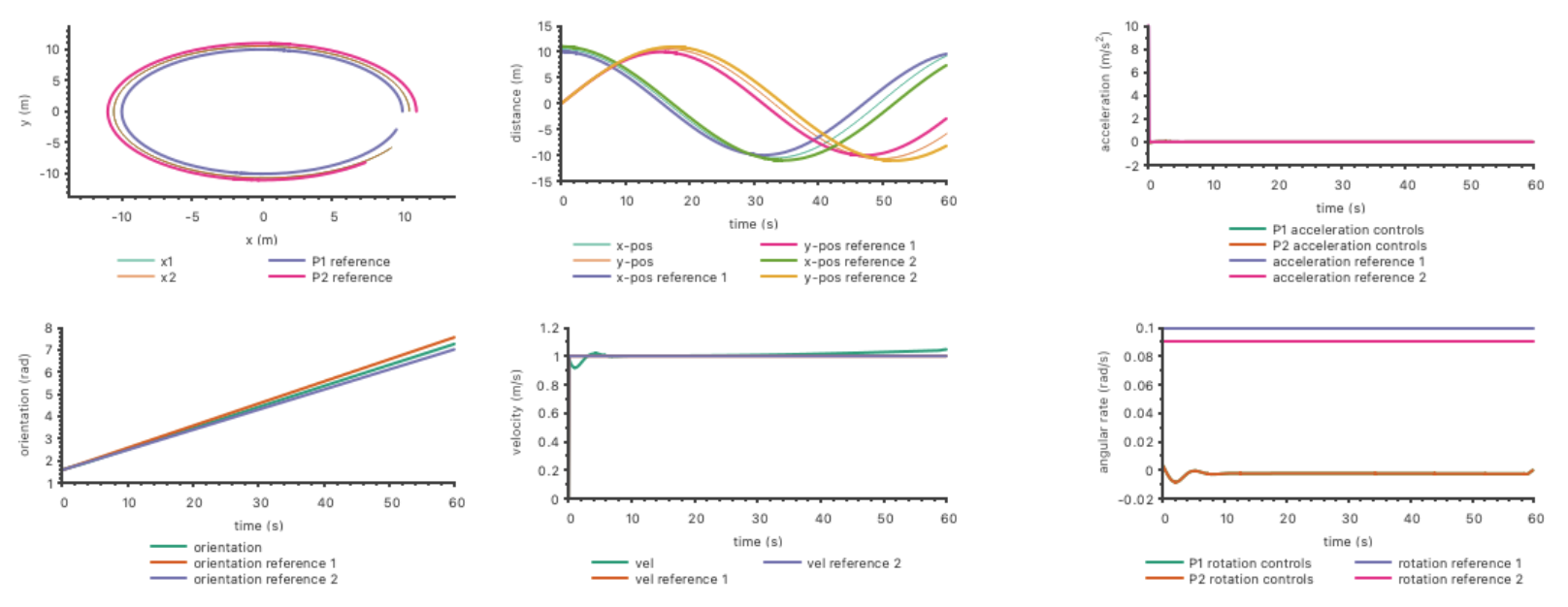
Note that the solution trajectory converges to be closer to the outer trajectory. Since the control costs are equal, this is expected because it takes less control effort to circle at a larger radius than a smaller one.
Stackelberg Game Formulation
Dextreit and Kolmanovsky 2014 introduce a Stackelberg game-theoretic controller which optimizes energy efficiency in a hybrid vehicle by modeling the human driver as a leader and the energy management system as a follower. The results suggest that Stackelberg games are well-suited for shared control applications.
For our project, we set up an LQ Stackelberg feedback game with nearly identical parameters to the LQ feedback Nash described previously. One difference of note was the introduce of the cross-control cost \( R^{12}_t \) as identity because the Stackelberg game required this cost to be positive definite.
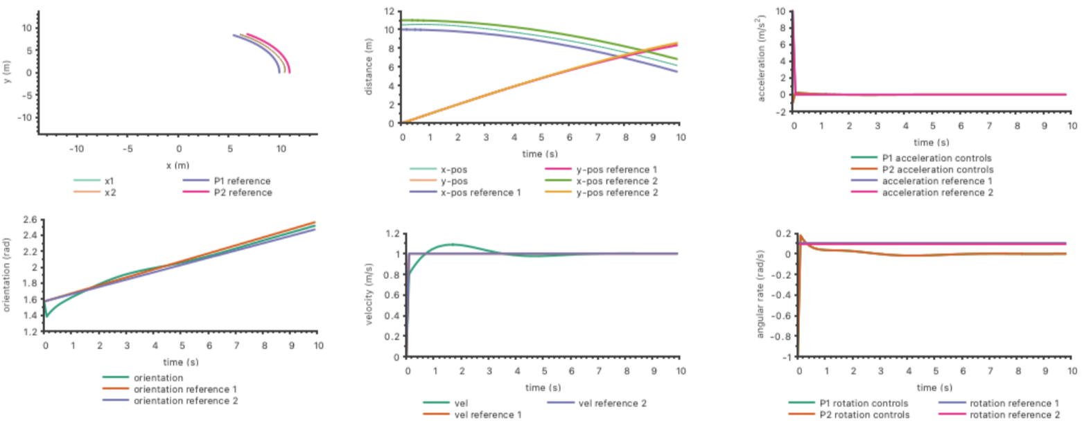
We present the following simulated results, which show the results for 100 time steps at 10 hertz (10 seconds). As implemented, the Stackelberg game showed instability if run too long and we are currently debugging the reason for this behavior. For these results, the leader seeks to follow a circle of radius 10 meters and the other 11 meters.
Bayesian Filter
Multiple model estimators use a bank of state estimators to estimate model probabilities. The state estimators each assume a different model and interact with one another via a cooperation strategy. Here, we had two models, with model \(i\) assuming control input \(\mathbf{u}_t^\left(i\right)\). The measurements were 2D positions at each timestep. We used a square root unscented Kalman filter (SR-UKF) as the state estimator and the simplest multiple model framework, autonomous multiple model (AMM) estimation. Under the AMM cooperation strategy, the SR-UKFs were run completely independently over all the measurements, and then the model probabilities were updated via Bayes’s rule:
\[\mu_{t+1}^{\left(i\right)}\propto\mu_t^{\left(i\right)}g_t\!\left(z_t\;\middle|\;\hat{\mathbf{x}}_{\left.t+1\middle|t\right.}^{\left(i\right)}\right)\,\]where \(\mu_t^{\left(i\right)}\) is the probability of model \(i\) being correct and \(g_t\) is the measurement likelihood given the prior state estimate \( \hat{\mathbf{x}}_{\left.t+1 \mid t\right.}^{(i)} \).
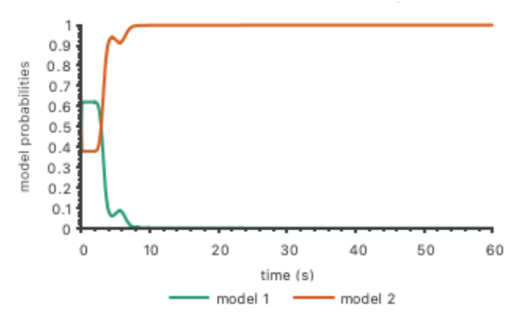
In the following figure, we show the Bayesian filter running on two models of behavior for the Nash game, one which seeks to follow a circle of radius 10 meters and the other 11 meters.
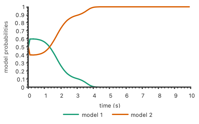
Next, we show the Bayesian filter running on two models of behavior for the Stackelberg game set up as described in that section. Once again, the leader seeks to follow a circle of radius 10 meters and the follower a circle of 11 meters.
Hardware Implementation on DeepRacer
A Vicon motion capture system was used to get position, base orientation, and velocity data at 100 Hz. Once the vehicle started moving, orientation was calculated based on the 2D velocity. In order to transform the control inputs from angular rate (\(\omega\)) and acceleration (\(a\)) to steering angle (\(\psi\)) and throttle (\(\tau\)), quadratic approximations were calculated:
\[\psi=w^{\mathsf{T}}Aw+Bw+C\,,\]where \(w=\left[\omega ~~ v\right]^{\mathsf{T}}\), and
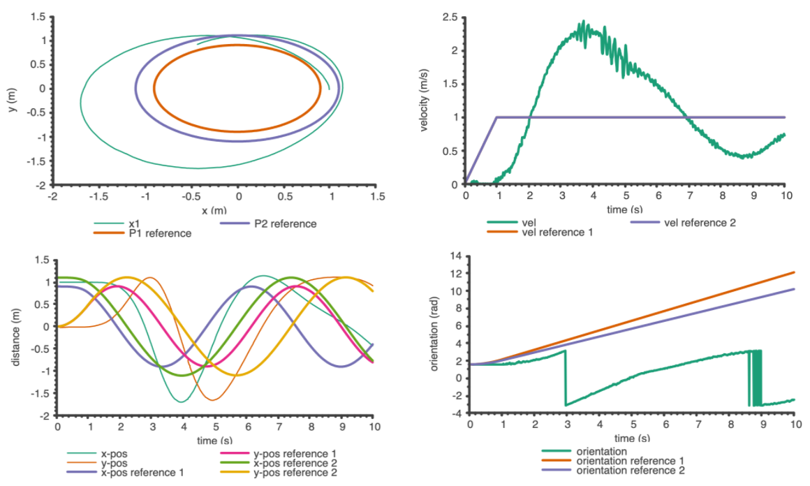
\[v=c_2\tau^2+c_1\tau+c_0\implies a=2c_2\tau\dot{\tau}+c_1\dot{\tau}\implies\Delta\tau=\frac{a\Delta t}{2c_2\tau+c_1}\,.\]We demonstrated the Nash game described above on the vehicle, with reduced radii, increased frequency, and a longer initial acceleration phase to make it tractable. As the results show, the hardware test was qualitatively similar to the simulation, but with significant overshoot and oscillation in velocity. This was likely due to the throttle model being calibrated only at steady-state and not accounting for static friction at low velocities.
Future Work
The work described was completed by Benjamin Reifler and Hamzah Khan at the University of Texas at Austin for the Modeling Multi-Agent Systems course in Fall 2021.
- Fix Stackelberg simulation.
- Design and run experiments with human in the loop to expose limits.
- Consider more interesting reference trajectories than circles of different radii.
- Include constraints in game formulation.
- Explore potential divergence between error states and look into model-predictive control.
Works Cited
C. Dextreit and I. V. Kolmanovsky. Game theory controller for hybrid electric vehicles. IEEE Transactions on Control Systems Technology, 22(2):652–663, 2013.
B. N. Patel, L. Rosenberg, G. Willcox, D. Baltaxe, M. Lyons, J. Irvin, P. Rajpurkar, T. Amrhein, R. Gupta, S. Halabi, C. Langlotz, E. Lo, J. Mammarappallil, A. J. Mariano, G. Riley, J. Seekins, L. Shen, E. Zucker, and M. P. Lungren. Human–machine partnership with artificial intelligence for chest radiograph diagnosis. npj Digital Medicine, 2(1):111, 2019. doi: 10.1038/s41746-019-0189-7. URL https://doi.org/10.1038/s41746-019-0189-7.
F. Flemisch, D. Abbink, M. Itoh, M.-P. Pacaux-Lemoine, and G. Weel. Shared control is the sharp end of cooperation: Towards a common framework of joint action, shared control and human machine cooperation. IFAC-PapersOnLine, 49(19):72–77, 2016. ISSN 2405-8963. doi: https://doi.org/10.1016/j.ifacol.2016.10.464. URL https://www.sciencedirect.com/science/article/pii/S2405896316320547. 13th IFAC Symposium on Analysis, Design, and Evaluation ofHuman-Machine Systems HMS 2016.
D. H. Klyde, P. C. Schulze, D. Mitchell, and N. Alexandrov. Development of a process to define unmanned aircraft systems handling qualities. In 2018 AIAA Atmospheric Flight Mechanics Conference, page 0299, 2018.